The inspiration for this blog stems from a discussion I had with a James - a Tech Fellow from Goldman Sachs(not outing his full name here) who primarily works on HPC and file systems. The context of this conversation was what he looks for in candidates applying to be a part of his team and what usually stands out.

His advice - BREAK THINGS

“Break things every chance you get. You are not learning anything until you push these systems to their absolute limit. There is a certain amount of knowledge synthesis that happens at this stage, when you know WHY a system breaks or WHY it doesn’t”

At uni, we’re often taught to analyze algorithms using the Big O notation. An algorithm that is O(n) is better than one that is O(n²), and we strive to find the most efficient algorithm in terms of its asymptotic complexity. But what happens when two algorithms have the same complexity? Are they always equally fast?

The answer, perhaps surprisingly, is no. In this post, we’ll explore a fascinating example that demonstrates how the underlying hardware, specifically the CPU cache, can have a dramatic impact on performance. We’ll look at two O(n²) algorithms for traversing a 2D matrix and see why one is significantly faster than the other, thanks to a concept called cache locality.

Asymptotic Analysis: A Quick Refresher

Asymptotic analysis, or Big O notation, is a way to describe the performance of an algorithm as the input size grows. It gives us a high-level understanding of how an algorithm scales. For example, an O(n²) algorithm’s runtime will grow quadratically with the input size n.

While incredibly useful, Big O notation deliberately ignores constants and lower-order terms. It doesn’t care about the exact number of operations, but rather the growth rate. This means that two O(n²) algorithms might have very different constant factors, leading to different real-world performance.

The Memory Hierarchy and Cache Locality

Modern computers have a memory hierarchy. At the top, we have CPU registers, which are extremely fast but very small. Then we have multiple levels of cache (L1, L2, L3), which are progressively larger but slower. Finally, we have the main memory (RAM), which is much larger but also much slower than the cache.

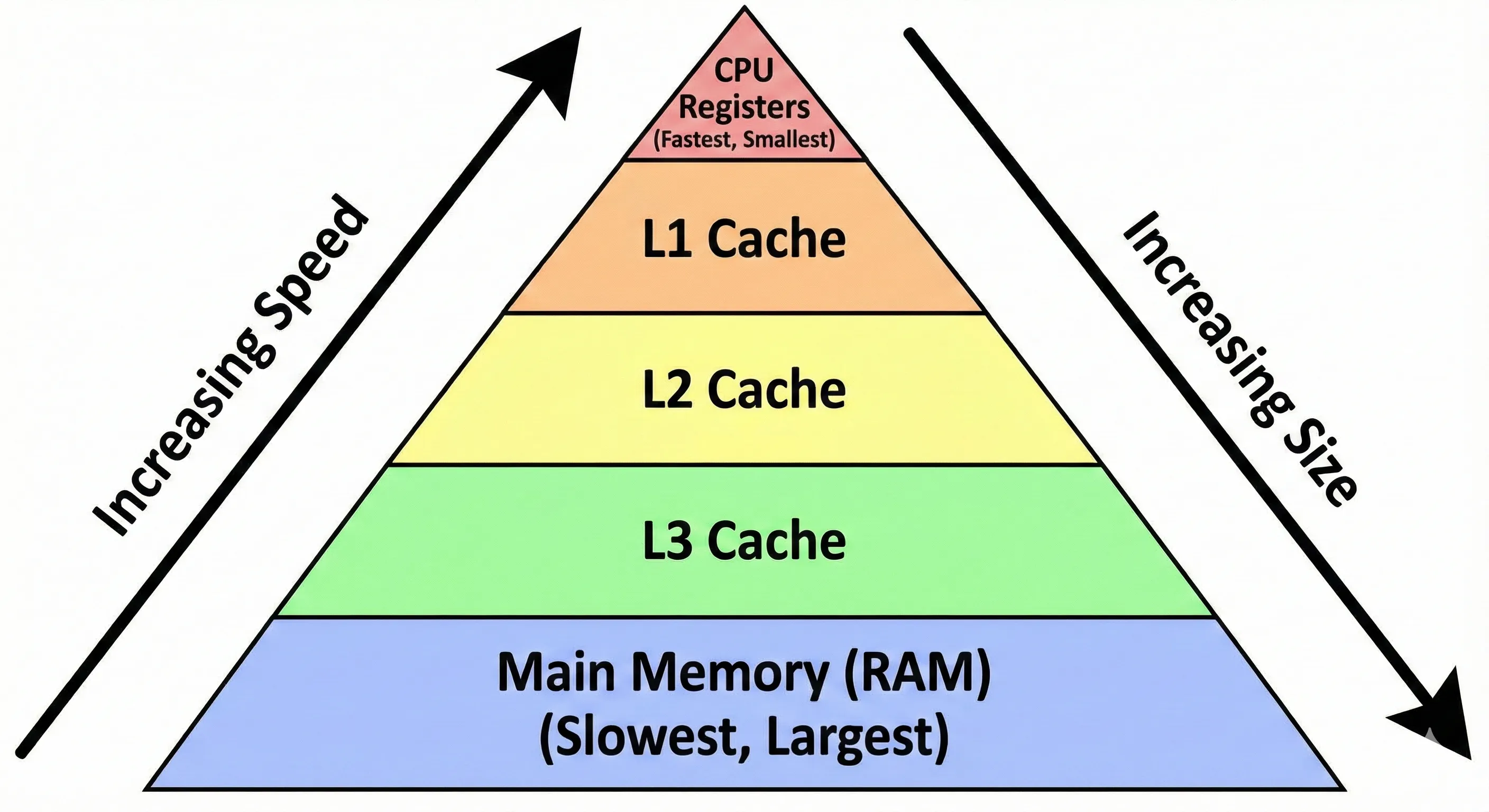Image Credits - Nano Banana Pro

When the CPU needs to access data, it first checks the L1 cache. If the data is there (a cache hit), it’s accessed very quickly. If not (a cache miss), the CPU checks the L2 cache, then L3, and finally RAM. Each level of miss incurs a significant performance penalty.

To minimize cache misses, modern CPUs are designed to exploit two principles of locality:

• Temporal Locality: If a piece of data is accessed, it’s likely to be accessed again soon.
• Spatial Locality: If a piece of data is accessed, it’s likely that data near it in memory will be accessed soon.

When a cache miss occurs, the CPU doesn’t just fetch the single piece of data it needs from RAM. It fetches a whole block of contiguous data (called a cache line) and stores it in the cache, anticipating that nearby data will be needed soon. This is where our 2D matrix example comes in.

The 2D Matrix Traversal Problem

Let’s consider a simple task: summing all the elements in a large 2D matrix. We can do this in two ways:

1. Row-major traversal: Iterate through each row, and for each row, iterate through its columns.
2. Column-major traversal: Iterate through each column, and for each column, iterate through its rows.

Here’s how you might write this in Python using NumPy:

import numpy as np

# Create a large 10000x10000 matrix
matrix = np.ones((10000, 10000))

def sum_row_major(matrix):
    total = 0
    for i in range(matrix.shape[0]):
        for j in range(matrix.shape[1]):
            total += matrix[i, j]
    return total

def sum_column_major(matrix):
    total = 0
    for j in range(matrix.shape[1]):
        for i in range(matrix.shape[0]):
            total += matrix[i, j]
    return total

Both of these functions have two nested loops, each running n times (where n is the dimension of the matrix). Therefore, both have a time complexity of O(n²). Asymptotically, they are identical. But in practice, their performance is anything but.

The Performance Difference: It’s All About the Cache

2D arrays are typically stored in memory in row-major order. This means that the elements of the first row are stored contiguously in memory, followed by the elements of the second row, and so on. 2D arrays are typically stored in memory in row-major order. This means that the elements of the first row are stored contiguously in memory, followed by the elements of the second row, and so on.

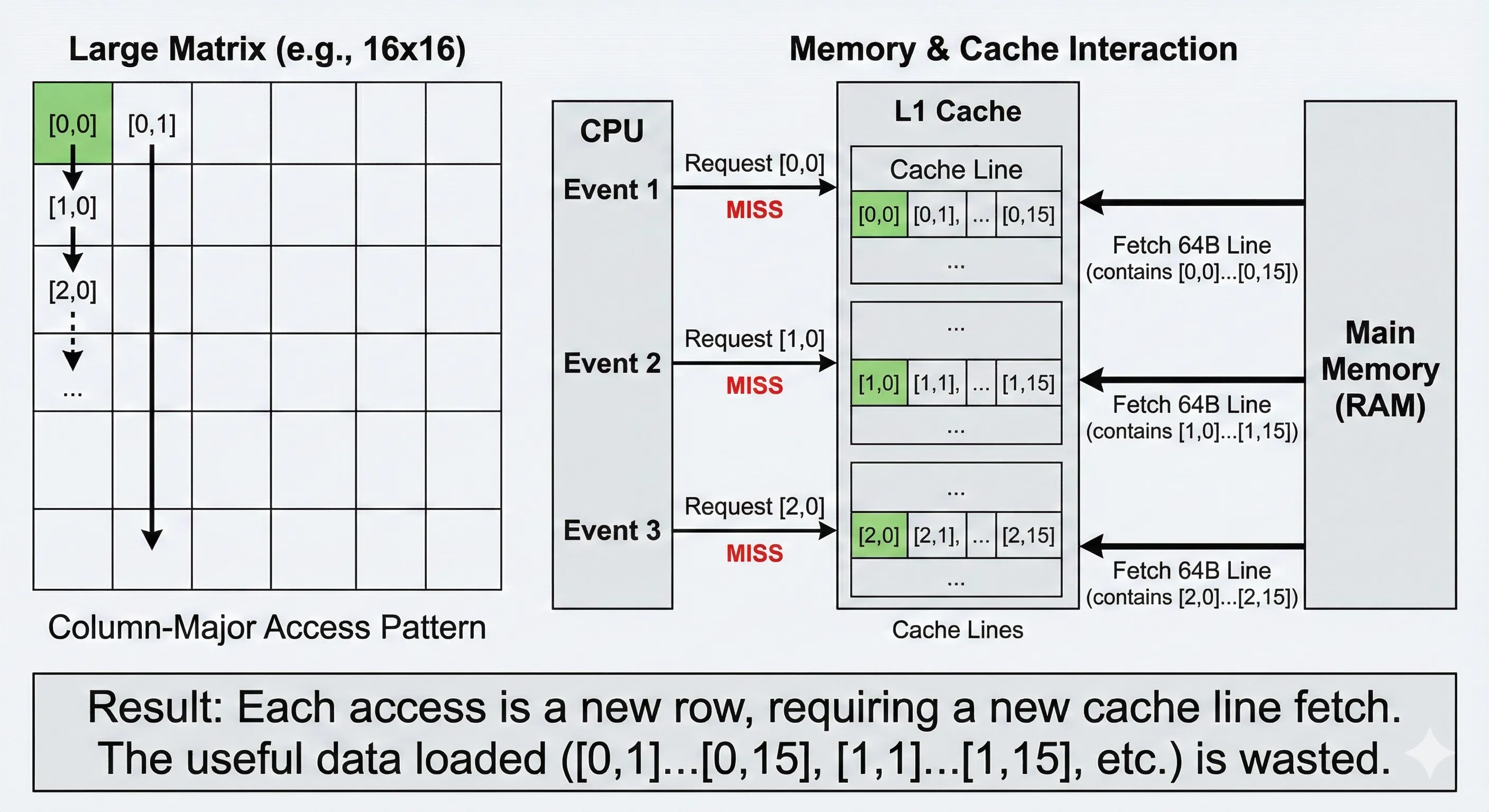Image Credits - Nano Banana Pro

Row-major traversal accesses the elements in the exact order they are laid out in memory: matrix[0,0], matrix[0,1], matrix[0,2], … This is a perfect example of spatial locality. When the CPU fetches the first element, it also loads the next few elements into the cache line. Subsequent accesses are then lightning-fast cache hits.

Column-major traversal, on the other hand, jumps around in memory. It accesses matrix[0,0], then matrix[1,0], then matrix[2,0], etc. These elements are far apart in memory (separated by the length of a full row). Each access is likely to result in a cache miss, forcing the CPU to go all the way to RAM, which is orders of magnitude slower.

Let’s Benchmark It

Now of course, the previous section showed you a Python code snippet but we will not using it for this experiment. Primiarly because, if you ran the previous code, you will see that there is no difference between the two algos. They both take really realy long lol - the bottleneck here comes from Python’s typechecking and other library level implementations.

I will probably plan another blog to expand more on a Python specific differences for this algo :)

A C++ Demonstration

The effect is even more pronounced in a language like C++ where we have more direct control over memory.

#include <iostream>
#include <vector>
#include <chrono>

const int SIZE = 10000;

using namespace std;  //to make the code less cluttered hehe

int main() {
    vector<vector<int>> matrix(SIZE, vector<int>(SIZE, 1));

    // Row-major traversal
    auto start = chrono::high_resolution_clock::now();
    long long sum1 = 0;
    for (int i = 0; i < SIZE; ++i) {
        for (int j = 0; j < SIZE; ++j) {
            sum1 += matrix[i][j];
        }
    }
    auto end = chrono::high_resolution_clock::now();
    chrono::duration<double> row_duration = end - start;
    cout << "Row-major traversal time: " << row_duration.count() << "seconds" << endl;


    // Column-major traversal
    start = chrono::high_resolution_clock::now();
    long long sum2 = 0;
    for (int j = 0; j < SIZE; ++j) {
        for (int i = 0; i < SIZE; ++i) {
            sum2 += matrix[i][j];
        }
    }
    end = chrono::high_resolution_clock::now();
    chrono::duration<double> col_duration = end - start;
    cout << "Column-major traversal time: " << col_duration.count() << " seconds" << endl;

    cout << "Difference: Column-major is " << col_duration.count() / row_duration.count() << "x slower" << endl;

    return 0;
}

Conclusion

Asymptotic analysis is a fundamental tool for algorithm design, but it’s not the whole story. Understanding how your code interacts with the underlying hardware can lead to significant performance improvements. The 2D matrix traversal example is a classic demonstration of how a simple change that respects cache locality can make an O(n²) algorithm dramatically faster than another O(n²) algorithm.

So next time you’re optimizing a piece of code, don’t just think about the Big O. Think about the memory access patterns too. You might be surprised at the performance gains you can achieve.